I’ve blogged a lot about various cognitive biases and logical fallacies here over the years, but today I want to talk about one I just kinda made up: The Tim Tebow Fallacy. Yeah, that’s right, this guy:
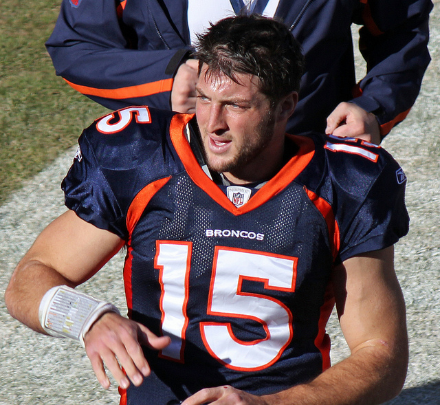
I initially mentioned the premise in this post, but for those of you who missed it here’s the background: Tim Tebow is a Heisman trophy winning quarterback who played in the NFL from 2010-2012. Despite his short career, in 2011 he was all anyone could talk about. Everyone had an opinion about him and he was unbelievably polarizing, despite being a quite pleasant individual and a good-but-not-great player. It was all a little baffling, and writer Chuck Klosterman took a crack at explaining the issue here. In trying to work through the controversy, he made this observation:
On one pole, you have people who hate him because he’s too much of an in-your-face good person, which makes very little sense; at the other pole, you have people who love him because he succeeds at his job while being uniquely unskilled at its traditional requirements, which seems almost as weird. Equally bizarre is the way both groups perceive themselves as the oppressed minority who are fighting against dominant public opinion, although I suppose that has become the way most Americans go through life.
Ever since I read that, I’ve been watching political conversations and am stunned how often this type of thinking happens. It seems some people not only want to have a belief and defend it, but also get some sort of cache from having an unacknowledged or rare belief. It’s like a combination of a reverse-Bandwagon effect (where someone likes something more because it’s not popular) combined with type of majority illusion (where people inaccurately assess how many people actually hold a particular opinion). So as a fallacy, I’d say it’s when you find a belief more attractive and more correct because it runs counter to what you believe popular perception is. To put it more technically:
Tim Tebow Fallacy: The tendency to increase the strength of a belief based on an incorrect perception that your viewpoint is underrepresented in the public discourse
Need an example? Take a group conversation at a party: Person A mentions they like the Lord of the Rings movies. Person B pipes up that they actually really didn’t like them. Person C agrees with Person B, and the two bond a bit over finding out they share this unusual opinion. After a minute or two, Person A is getting a little frustrated and is now even a BIGGER fan of the movies. If it stopped there it wouldn’t be a Tebow fallacy, just regular old defensiveness. What kicks it over the edge is when Person A starts claiming “no one ever talks about how good the cinematography was in those movies!” or “no one really appreciates how innovative those were!”. or “No one ever gives geeky stuff any credit!”. They walk away irritated and believing that saying you like the Lord of the Rings movies has been sort of a subversive act, and that general defensiveness is called for.
Now of course this is all kind of poppycock. The Lord of the Rings movies are some of the most highly regarded movies of all time, and set records for critical acclaim and box office draw. The viewpoint Person A was defending is the dominant one in nearly every circle except for the one they happened to wander in to that night, yet they’re defensive and feel they need to continue to prove their point. It’s the Tim Tebow Fallacy.
Now I think there’s a couple reasons this sort of thing happens, and I suspect many of them are getting worse because of the internet:
- We’re terrible at figuring out how widespread opinions are. In my Lord of the Rings example, Person A extrapolated small group dynamics to the general population, likely without even realizing it. Now this is pretty understandable when it happens in person, but it gets really hard to sort through when you’re reading stuff online. Online you could read pages and pages of criticism of even the most well-loved stuff, and come away believing many more people think a certain way than they do. Even if 99.9% of American love something that still leave 325,000 who don’t. If those people have blogs or show up in comments sections, it can leave you with the impression that their opinions are more widely held than they are. And make no mistake, this influences us. It’s why Popular Science shut off their comments section.
- We feed off each other and headlines The internet being what it is, let’s imagine Person A goes home and vents their frustrations with Person B and C online. What started as an issue at one party no turns in to an anecdote that can be spread. The effect of this should not be underestimated. A few months ago someone sent me this story, about a writer with a large-ish Twitter following who had Tweeted a single picture of a lipstick name “Underage Red” with the caption “Just went shopping for some makeup. How is this a lipstick color?”. The whole story is here, but by the end of it her single Tweet had made it all the way to Time Magazine as proof of a “major controversy” and being cited as an example of “outrage culture”. She was inundated with people calling her out (including the lipstick creator, Kat Von D) for her opinion, all seemingly believing they were fighting the good fight against a dominate narrative. A narrative that was comprised of a single rather reasonable Tweet about a lipstick. I don’t blame those people by the way….I blame the media that creates an “outrage” story out of a single Tweet, then follows up with think pieces about “PC culture” and “oversensitivity”. The point is that in 2016, a single anecdote going viral is really common, but I’m not sure we’ve all adjusted our reactions to account for the whole “wait, how many people actually think this way?” piece. It’s even worse when you consider how often people lie about stuff. Throw in a few fabricated/exaggerated/one sided retellings, and suddenly you can have viral anecdotes that never even happened.
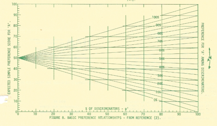
- It’s human nature to strive for optimal distinctiveness. While going with the crowd gets a lot of attention, I think it’s worth noting that humans actually are a little ambivalent about this. The theory of optimal distinctiveness argues that we actually are all simultaneously striving to differentiate ourselves just enough to be recognized while not going so far as to be ostracized. Basically we want to be in the middle of this graph:

From Brewer, M.B. (1991). “The social self: On being the same and different at the same time”. Personality and Social Psychology Bulletin, 17, 475-482.
By positioning our arguments against the dominant narrative, we can both defend something we really believe in AND differentiate ourselves from the group. I think that makes this type of fallacy uniquely attractive for many people.
- We’re selecting our own media sources, then judging them. One of my favorite humor websites of all times is Hyperbole and a Half by Allie Brosh. After going viral, Brosh put together an FAQ that includes this question/answer:
Question: I don’t think you’re funny and I’m frustrated that other people do Answer: It’s okay. Try not to be too upset about it. Humor is simply your brain being surprised by an unexpected variation in a pattern that it recognizes. If your brain doesn’t recognize the pattern or the pattern is already too familiar to your brain, you won’t find something humorous.
With the internet (and cable news, Facebook, Twitter, etc) we now have the ability to see hundreds or thousands of different opinions in a single week. What we often fail to recognize is that we actually select for most of these….who we follow or friend, webpages we visit etc. Everyone else does too. We are all constructing very individualized patterns of information intake, and it’s hard to know how usual or unusual our own pattern is. Instead of just “those who loved Lord of the Rings movies” and “those who didn’t” there’s also “those who hated it because they are huge book fans”, “those who don’t like any movie with magic in it”, “those who hated it because they hate Elijah Wood”, “those who prefer Meet the Feebles”, “those who didn’t get that whole ring thing”, “those who thought that was the one with the lion”, “those who liked it until they heard all the hype then wished everyone would calm down”, etc etc etc. Point is, we are often selecting for certain opinions, then reacting to the opinions we selected ourselves and taking it out on others who may legitimately never have encountered the opinion we’re talking about. If you combine this with point #3 above, you can see where we end up positioning ourselves against a narrative others may not be hearing.
- It’s a common mistake for great thinkers. Steve Jobs is widely considered one of the most innovative and intuitive businessmen of all time. His success largely came from his uncanny ability to identify gaps in the tech marketplace that were invisible to everyone else and then fill them better than anyone. What often gets lost in the quick blurbs about him though is how often he misfired. He initially thought Pixar should be a hardware company. He wiffed on multiple computer designs and had a whole confusing company called NeXT…..and he’s still considered one of the best in the world at this. Great thinkers are always trying to find what others are missing, and even the best screw this up pretty frequently. As with many fallacies, it’s important to remember that IQ points offer limited protection. What makes your mind great can also be your downfall.
- It gets us out of dealing with uncomfortable truths. One of the first brutal call outs I ever got on the internet was a glib and stupid comment I made about the Iraq War. It was back in 2004 or so, and I got in an argument with someone I respected over whether or not we should have gone in. I was against the war, and at some point in the debate I got mad and said that my issue was that George Bush “hadn’t allowed any debate”. I was immediately jumped on and it was pointed out to me in no uncertain terms that I was just flat out making that up. There was endless debate, I just didn’t like the outcome. That stung like hell, but it was true. Regardless of what anyone believes about the Iraq War then or now, we did debate it. It was easier for me to believe that my preferred viewpoint had been systematically squashed than that others had listened to it and not found it compelling. This works the other way too. I’m sure in 2004 I could find someone claiming vociferously that we’d over-debated the Iraq War, based mostly on the fact that they made up their mind early. Most recently I saw this happen with Pokemon Go, where the Facebook statuses talking about how great it was showed up about 30 minutes before the “I’m totally sick of this can we all stop talking about this” statuses showed up. I’m not saying there’s a “right” level of public discourse, but I am saying that it’s hard to judge a “wrong” level without being pretty arbitrary. We all want the game to end when our team’s ahead, but it really just doesn’t work that way.
So that’s my grand theory right there. As I hope point #6 showed, I don’t think I’m exempt from this. A huge amount of this blog and my real life political discussion are based on the premise of “not enough people get this important fact I’m about to share”. I get it. I’m guilty.
On the other hand, I think in the age of the internet when we can be exposed to so many different viewpoints, we should be careful about how we let the existence of those viewpoints influence our own feelings. If the forcefulness of our arguments is always indexed on what we think the forcefulness of our opposition is, that will leave us progressively more open to infection by the Toxoplasma of Rage. As the opportunities for creating our own “popular narrative” increase, we have to be even more careful that we reality check that at times. Check the numbers in opinion polls. Read media that opposes you. Make friends outside your demographic. Consider criticism. Don’t play for the Jets. You know, all the usual fallacy stuff.
Tebow Image Credit