In honor of the New Year and New Year’s Resolutions and such, I’m trying out a different type of post today. This post isn’t about statistical theory or stats in the news, but actually about how I personally use data in my daily life. If you’re not particularly interested in messy data, personal data, or weight loss, I’d skip this one.
Ah, it’s that time of year again! The first day of 2017, a time of new beginnings and resolutions we might give up by February. Huzzah!
I don’t mean to be snarky about New Year’s Resolutions. I’m actually a big fan of them, and tend to make them myself. I’m still trying to figure out some for 2017, but in the meantime I wanted to comment on the most common New Year’s Resolution for most people: health, fitness, and weight loss. If Mr Nielsen there is to be believed, a third of Americans resolve to lose weight every year, and another third want to focus on staying fit and healthy. It’s a great goal, and one that is unfortunately challenging for many people. It seems there are a million systems to advise people on nutrition, exercise plans and other such things, and I am not about to add anything to that mix. What I do have however is my own little homegrown data project I’ve been tinkering with for the last 9 months or so. This is the daily system I use to help me work on my own health and fitness by using my own data to identify challenges and drive improvements. While it certainly isn’t everyone’s cup of tea, I’d gotten a few questions about it IRL, so I thought I’d put it up for anyone who was interested in either losing weight or just seeing the process.
First, some personal background: Almost exactly 2 years ago (literally: December 31st, 2014), I decided to start meeting with a nutritionist to help me figure out my diet and lose some weight. Like lots of people who have a lot on their plate (pun intended), I had a ridiculous amount of trouble keeping my weight in a healthy range. The nutritionist helped quite a bit and I made some good progress (and lost half the weight I wanted to!), but I realized at some point I would have to learn how to manage things on my own. Having an actual person track what you are doing and hold you accountable is great and was working well, but I wanted something I could keep up without having to make an appointment.
Now, the math background: Around the same time I was pondering my weight loss/nutritionist dilemma I got asked to give a talk at a conference on the topic “What Gets Measured Gets Managed”. One of the conference organizers had worked with me a few years earlier and said “I know you were always finding ways of pulling data to fix interesting problems, do you have anything recent you’d like to present?” Now this got me thinking about my weight. How was it that I could always find a data driven way to address a work problem, but couldn’t quite pull it together for something important to me in my personal life? I had tried calorie counting in the past, and I had always gotten frustrated with the time it took and the difficulty in obtaining precise measurements, but what if I could come up with some simpler alternative metrics? With my nutritionists blessing (she had a remarkable tolerance for my love of stats), I decided to work on it.
The General Idea: Since calories were out, I decided to play around with the idea of giving myself a general “score” for a day. If I could someone capture a broad range of behaviors that contributed to weight gain and the frequency in which I engaged in them, I figured I could figure out exactly what my trouble spots were, troubleshoot more effectively and make sure I stayed on track. At the end of each week I’d add up my weekly score and weigh myself. If I lost weight, no problem. If I gained weight, I’d tweak things.
The Categories: The first step was to come up with categories that covered every possible part of my day or decision I felt contributed noticeably to my weight. I aimed for 10 because base 10 rules our lives. My categories fell in to four types:
- Meals and snacks I eat 3 meals and 2 snacks each day, so each got their own category.
- Treat foods Foods I need to watch: sweets/desserts, chips, and alcohol each got their own category
- Health specific issues I have celiac disease and have to avoid gluten. Since eating gluten seems to make me either ridiculously sick or ravenously hungry, I gave it a category so I could note if I thought I got exposed
- Healthy behaviors I ultimately only track exercise here, but I have considered adding sleep or other non-food behaviors too.
The Scores: Each score ranges from 0 to 5, with zero meaning “perfect, wouldn’t change a thing” and five meaning “gosh, that was terribly ill-advised”. Between those two extremes, I came up with a slightly different scoring system for each category.
- Meals and snacks Basically how full I feel after I eat. I lay out a reasonable serving or meal beforehand, and then index the score from there. If I take an extra bite or two because the food just tastes good, I give myself a 1. If I was totally stuffed, it’s a 5. Occasionally I’ve even changed my ranking after the fact when I get to the next meal and discover I’m not hungry.
- Treat foods One serving = 1 point, 2 servings = 3 points, more than that is 4 or 5. The key here is serving. Eating a bunch of tortilla chips before a meal at a mexican restaurant is almost never one serving, and a margarita at the same restaurant is probably both alcohol and sugar. It helps to research serving sizes for junk food before attempting this one.
- Health specific issues For gluten, if I think I got a minor exposure, it’s a 1. The larger the exposure I got, the higher the ranking I give it. The day I got served a hamburger with what was supposed to be a gluten free only to discover it wasn’t? Yeah, that’s a 5.
- Exercise I generally map out my workouts for the week, then my score is based on how much I complete. A zero means I did the whole thing, a 5 means I totally skipped it. I like this because it incentivizes me to start a workout, even if I don’t finish it.
With 10 categories ranked 0 to 5, my daily score would be somewhere between 0 “perfect wouldn’t change a thing” and 50 or “trying to re-enact the gluttony scene from Seven“. To start, I figured I’d want to be below a score of 5 per day or 35 per week. Since I am not built for suffering, that seemed manageable.
Obviously all of those scores are a bit of a judgment call. If I lose track of what I ate or feel unhappy with it, I give myself a 5. I try not to over think these rankings to much, and just go with my gut. That mexican meal with the chips and margarita for example was a 5 for the chips, 3 for feeling full after dinner, 1 for the alcohol and 1 for the sugary margarita. Is that 100% accurate? Doubtful, but does a score of 10 seem about right for that meal? Sure. Will my scale be lower the day after a meal like that? No. A score of 10 works. With the categories and the score, my weekly spreadsheets end up looking like this:

How I use this data: Okay, so remember how I started this with “what gets measured gets managed”? I use this data to find weak spots, figure out where I’m having the most trouble, and to come up with solutions. For example, every month I add my scores up and figure out which category is my worst one. When I first started, I realized that I actually skipped a lot of workouts. When I looked at the data, I noticed that I would have one good week of working out followed by one bad week. When I thought about it, I realized I was trying to complete really intense workouts, and that I was basically burning myself out and needing to take a week off to regroup. When I decided to actually decrease the intensity of my workout plan, I stopped skipping days. Since the workout you actually do tends to be better than the one you only aspire to do, this was a win. Another trend I noted was that I frequently overate at dinner. This was solved by packing a bigger lunch. There’s a few other realizations like this, and they all had pretty simple fixes. For January I’m working on reducing the number of chips I eat, because damn can I not eat chips in moderation.
The results: So has this worked? Yes! Since April, I’ve lost almost 5 points off my BMI, which takes me from the obese/overweight line to the healthy/overweight line. Here’s my 7 day moving average (last 7 days averaged together) score plotted against a once a week weigh in. The red line is my goal of 5:
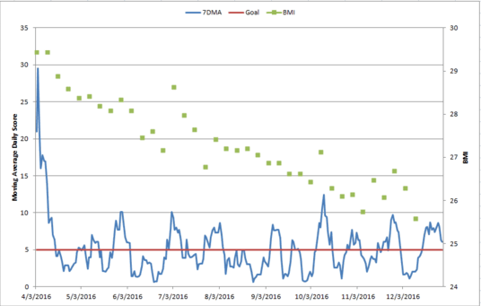
Note: There are some serious jumps on this chart, mostly because I can retain a crazy amount of water if I eat too much sodium.
At the moment I’ve decided to give myself a month off from weigh-ins since the holidays can be so crazy, but on that last weigh in I was only 3 lbs away from being in the normal BMI range. As I mentioned, I’m not built for suffering. Slow weight loss is fine with me.
It’s interesting to note that I actually don’t make my goal of 5 or less per day all the time. Over the 274 days I’ve been tracking, I only was at 5 or under about 70% of the time. I still lost weight. I’ve thought about raising my limit and trying to stay under it all the time, but as long as this is still working I’m going to stick with it.
General thoughts: Much of the philosophy behind how I pulled this data actually comes from the quality improvement “good enough” world, as opposed to the hard research “statistical significance” world. The weigh in data is always there to test my hypotheses. If my scoring system said I was fine but my weight was going up, I would change it. I’m sure that I have not accurately categorized every day I’ve had since April, but as long as my daily scores are close enough to reality, it works. It’s the general trend of healthy behaviors that matters, not any individual day. The most important information I’ve gotten out of this process is what small tweaks I can make to help myself be more healthy. Troubleshooting the life I actually have a getting specific feedback about which areas I have problems with has been immensely helpful. Too often health and diet advice advises us to impose Draconian limits on ourselves that set us up for failure. By tracking specific behaviors and tweaks over the course of months, it’s a lot easier to figure out the high impact changes we can make.
If I had any advice for anyone wanting to try a similar system, it would be to really customize the categories you track and to think through a ranking system that makes sense to you. Once I invented my system, I actually only have to spend about 45 seconds a day ranking myself. I only change things if I see the weight creeping up or if some piece seems to not be working. At this point I review the categories and scores monthly to see if any new patterns are emerging. In the quality improvement world, we call this a PDSA cycle: Plan, Do, Study, Act. Plan what you want to do, do what you said you would do, study what you did, act on the new knowledge. By having data on individual aspects of my daily life, this process became more manageable.
Happy tracking!


 This almost always gets a laugh, and most people then admit that it’s not the numbers they have a problem with, it’s the way they’re being used. There’s a lot of unpleasant news to deliver in this world, and people love throwing up numbers to absorb the pain. See, I would totally give you a raise or more time to get things done but the numbers say I can’t. When people know you’re doing exactly what you were going to do to begin with, they don’t trust any number you put up. This gets even worse in political situations. So please, for the love of God, if the numbers you run sincerely match your pre-existing expectations, let people look over your methodology, or show where you really tried to prove yourself wrong. Failing to do this gives all numbers a bad rap.
